Call Us:+1(928) 733-2150
In GASMOD Version 7.0, the pipeline model may be created graphically using a drag and drop approach. In this method, objects such as pipe segments, valves, tanks, compressor stations and other devices may be selected from a toolbox and dropped on a drawing canvas. These objects can be connected with pipe segments to form the pipeline system. The properties of each object may be defined by double-clicking on them and entering data in the screen that is displayed. A video tutorial is available that explains how the pipeline model can be created graphically.
These objects can be connected with pipe segments to form the pipeline system.
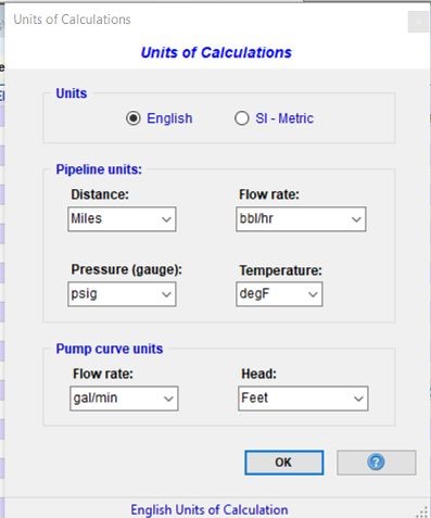
Initially, select the Units of Calculation(English/SI ) and select the objects to be included in the pipeline using the 5 steps to get started
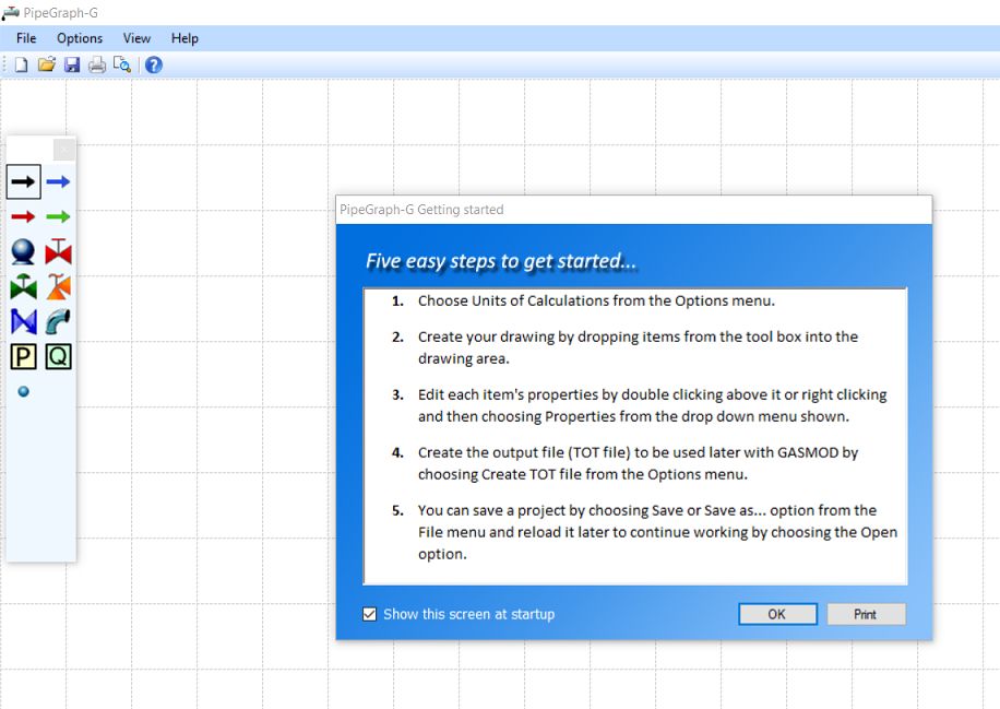
The properties of each object may be defined by double-clicking on them and entering data in the screen that is displayed. A video tutorial is available that explains how the pipeline model can be created graphically.
GasmodTutorial.jpg
GASMOD is a hydraulic simulation software for gas pipelines that takes into account the heat transfer between the gas in the pipeline and the surrounding medium. Gas may be injected or delivered at various locations along the pipeline. The resultant blended gas properties (specific gravity and viscosity) are calculated for each pipe segment at the flowing gas temperature. Multiple compressor stations along the pipeline may be modeled Calculations are performed for a given input flow rate and gas properties. Incoming and outgoing branch pipes and pipe loops at any location along the main pipeline may be specified. The ambient soil temperature and the pipe roughness may be varied along the pipeline. GASMOD can be used for the design of a new pipeline or checking capabilities of existing pipelines.
Pipeline profile data (distance, elevation, diameter, wall thickness, roughness etc.) along with all other data for a specific pipeline is stored in a file for future use. The built-in spreadsheet style data editor is used for creating a new pipeline data file. It features an easy to use spreadsheet data entry. All pipeline and branch pipe data files are created and edited using this spreadsheet editor. The input data consists of pipeline data, gas flow rate, compressor station data and thermal conductivity data for pipe and soil.
In each data entry screen, default data is provided in most cases. Help is available on each screen and on the status bar at the bottom of each data entry screen.
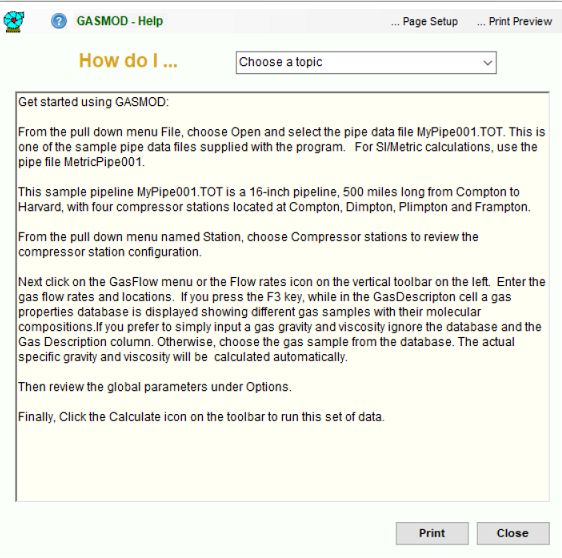
In addition, the How do I? screen steps you through the various options in the program as shown below
Calculations may be performed in English (US Customary Units) or SI (modified Metric) units.
The gas temperature and the pressure profile along the pipeline at the flow rates are calculated considering heat transfer with the surroundings. Using the input values of pipe, insulation and soil thermal conductivities, heat transfer and pressure drop calculations proceed along the length of the pipeline. The compressor horsepower required at each station is calculated considering the flow rate, suction and discharge pressures and compressor efficiency.
Creating a Pipeline Data File
You may create a new pipeline model by clicking the Graphic model button the left panel of the main GASMOD screen shown below. This approach allows you to pick various graphic objects, such as pipe segment, compressor station, valves, etc. from a toolbox and dropping them on a drawing area. Using pipe segments the objects are connected to form the pipeline. After building the graphic pipeline model the project can be saved. A GASMOD compatible data file (TOT file ) is automatically created. This is described in detail in several GASMOD Tutorial videos at SYSTEK's web site.
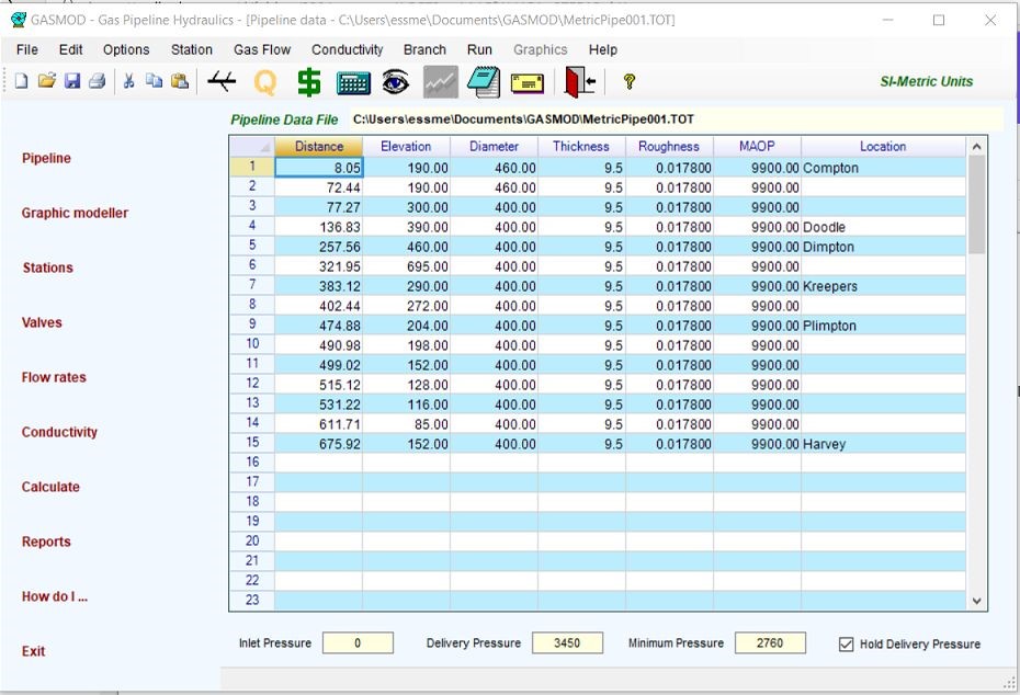
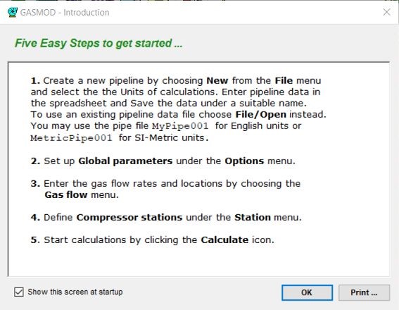
To create a pipeline model in a spreadsheet, choose File | New and follow the steps shown. To open an existing pipeline model, choose File | Open and choose the name of the pipe data file from the resulting screen. All pipe data files are designated with a file name extension of.TOT. Choosing the included sample pipeline MyPipe001 will display the data in the spreadsheet as shown below. This pipe data file contains all the information for the sample problem, described in the User Manual.
If a new pipeline data file is to be created from scratch, choose File | New and a blank spreadsheet screen will be presented for entering the pipeline data. After entering the pipeline data, save the file by selecting File | Save from the menu bar.
For further explanation on creating and editing pipeline data files, refer to the User Manual.
Each column in the spreadsheet is for a specific data for the pipeline. Each row represents a specific location along the pipeline. As the cursor (arrow) keys are moved around in the spreadsheet cells, the status bar at the bottom of the screen briefly describes the information to be entered in each cell. After each numeric entry, press Tab key or the arrow (cursor) key. The first column is for the distance measured from the origin of the pipeline, such as mile post. Each subsequent location of the pipeline is measured from the beginning of the pipeline and hence the first column is the cumulative length of each point on the pipeline measured from the beginning (where the inlet gas flow originates), also designated as mile post location (m.p.). Note that unlike other hydraulic simulation models, the distances are cumulative and not pipe segment lengths.
The second column is for the elevation of the pipe at that mile post location, measured above some datum, such as sea level. The third, fourth and fifth columns represent the pipe outside diameter, pipe wall thickness and the internal pipe roughness at this location. The pipe diameter, wall thickness and roughness entered at a specific location represent those for the pipe segment downstream of that milepost location. Thus, if the first two milepost locations are 0.0 and 45.0, as shown above, the diameter, wall thickness and roughness entered at 0.0 milepost are for the pipe segment from 0.0 to the 45.0 location. The diameter, wall thickness and roughness entered at milepost 45.0 are for the next pipe segment starting at milepost 45.0. Accordingly, for the very last milepost location, 420.0 (the last data row of the spreadsheet) the diameter, wall thickness and roughness entered should be a duplicate of the immediately previous location (milepost 380.0), since there is no pipe segment downstream of the last milepost. The pipe delivery pressure at the end of the pipeline and the minimum pressure required are input in the main screen. If a minimum delivery is to be held at the pipeline terminus, click the check box shown.
The next column entry is the maximum allowable operating pressure (MAOP) for the pipe at that milepost location. If you double-click with the cursor in the cell containing the MAOP, a data entry screen opens up. This screen can be used to verify or calculate the MAOP of the pipe. It also calculates the hydrostatic test pressures for pipe hoop stresses of 90% and 100% of the specified minimum yield strength (SMYS) of pipe material.
Note that for the pipeline profile, a maximum of 1000 points (or nodes) are allowed in the pipe data screen.
The pressure drop for each segment is calculated using the General flow equation and using friction factors calculated from Colebrook or AGA equations. Other flow equations, such as the Panhandle A and B, Weymouth, etc. are also available as options. A total of eight pressure drop equations are available to choose from. Pipeline elevations are also taken into account in determining the pressures along the pipeline.
Additionally, certain global data such as pressure drop formula, compressibility factor calculation method, maximum gas velocity, pipeline efficiency and gas specific heat ratio are also input. All input data are saved for the specific pipeline in a TOT file which is similar to an XML format. Thus a pipeline named Compton to Harvey will have all data stored in a file named ComptontoHarvey.TOT.
Entering Gas Properties, Pressures etc.
Next select Gas Flow from the icons or the menu bar. This screen lets you input distance, flow rate, specific gravity, viscosity and inlet temperature for the gas product that flows through the pipeline.
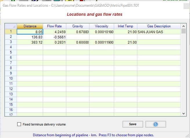
Gas flow data consists of the locations along the pipeline where gas is injected or delivered along with the gas specific gravity and viscosity. Optionally, the gas composition of each incoming gas stream may be specified. The program will calculate the gravity and viscosity of the gas from the compositional data. To specify a gas composition, press the F3 key with the cursor in the last column title GasDescription. This will display the available database containing various gases as shown.
Choosing a gas such as GULFCOAST and clicking OK will insert the gas title in theGasDescription column. The gas gravity and viscosity for this gas will be calculated and inserted in the third and fourth columns as shown below.
For specifying the thermal conductivity and pipe insulation data for heat transfer calculations, choose the Conductivity menu and the following screen is displayed. The thermal conductivity data includes thermal conductivity of pipe, insulation (if any) and soil in addition to the burial depth of pipe (cover) and ambient soil temperature. If the pipe is un-insulated, enter 0.0 for insulation thickness and the value of thermal conductivity of insulation is automatically ignored in the calculations.
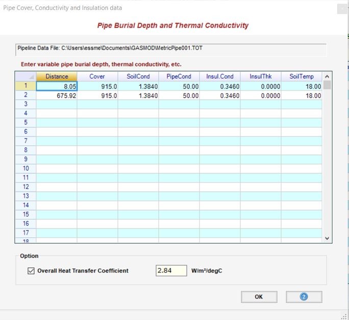
These values may be input as variable values along the length of the pipeline. Otherwise one row of data may be entered for the first pipeline node followed by one row of data for the last node as shown above. A fixed, overall heat transfer co-efficient may also be specified instead of the thermal conductivities. If the Overall Heat Transfer Coefficient box is checked, this value is used instead of calculating the heat transfer coefficient from the thermal conductivities.
For the sample problem, pipeline profile data (distance, elevation, pipe diameter and wall thickness, pipe roughness, MAOP) is saved in a file designated as MyPipe001.TOT. All other data for the specific pipeline such as thermal conductivity data, compressor station data, gas flow rate data etc. are also saved in the same text file named MyPipe001.TOT.
For specifying compressors along the pipeline, choose the Station menu followed Compressor Station option. The following screen is then displayed for entering the compressor station data.
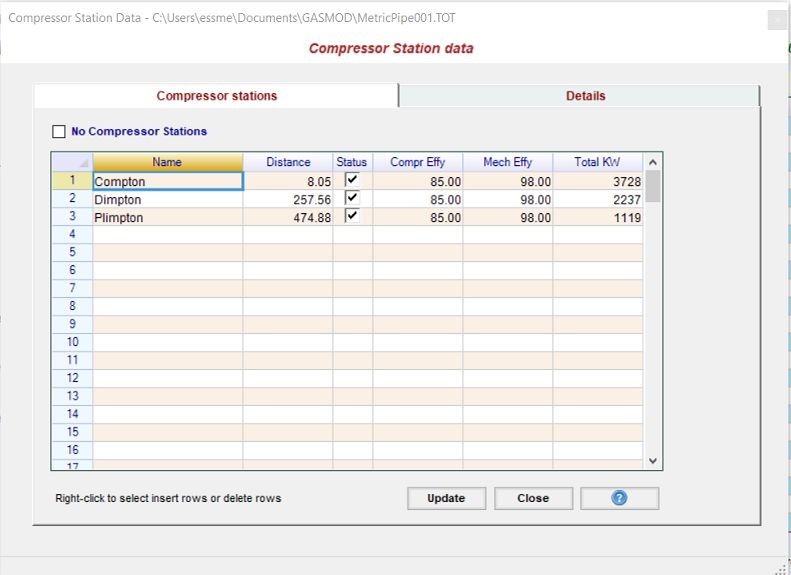
The compressor stations data consist of the locations, installed HP, suction and discharge pressures, suction and discharge losses as well as compressor adiabatic and mechanical efficiency. A maximum of 50 compressor station may be modeled.
The preliminary locations and number of compressor stations for a new pipeline may be determined approximately using the Locate Compressor Stations... option under the Stationmenu as shown below.
Choosing the Locate Compressor Stations... option, displays the following screen:
For a given pipe MAOP, gas inlet flow rate and allowable compression ratio, GASMOD will calculate the approximate locations of the required compressor stations.
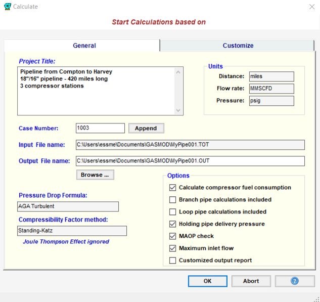
Next, click on the Calculator icon to start calculations. In the resulting screen enter the project title, case number, etc and select the necessary checkboxes. The project title may be entered as free flow text as shown. Notice that the pipe data file name and the corresponding output file names are shown as MyPipe001.TOT and MyPipe001.OUT respectively. If the input pipe data file were AGlobalPipeline.TOT, the corresponding results of calculation will be stored in a file named AGlobalPipeline.OUT.
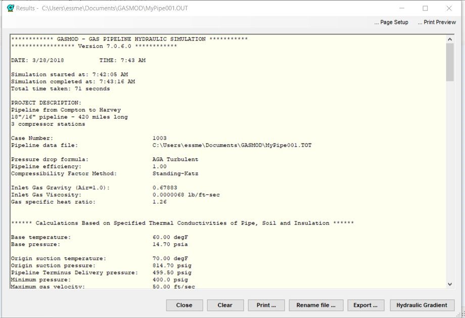
The calculated results are displayed on the screen, as well as saved in a file for later viewing or printing. A printed hard copy of the calculated results may be obtained by clicking the Print button below.
The output report consists of the flowing gas temperature, specific gravity, viscosity, and the pressures along the pipeline, along with the compressor suction and discharge pressures, horsepower(HP) and fuel consumption at each compressor station.
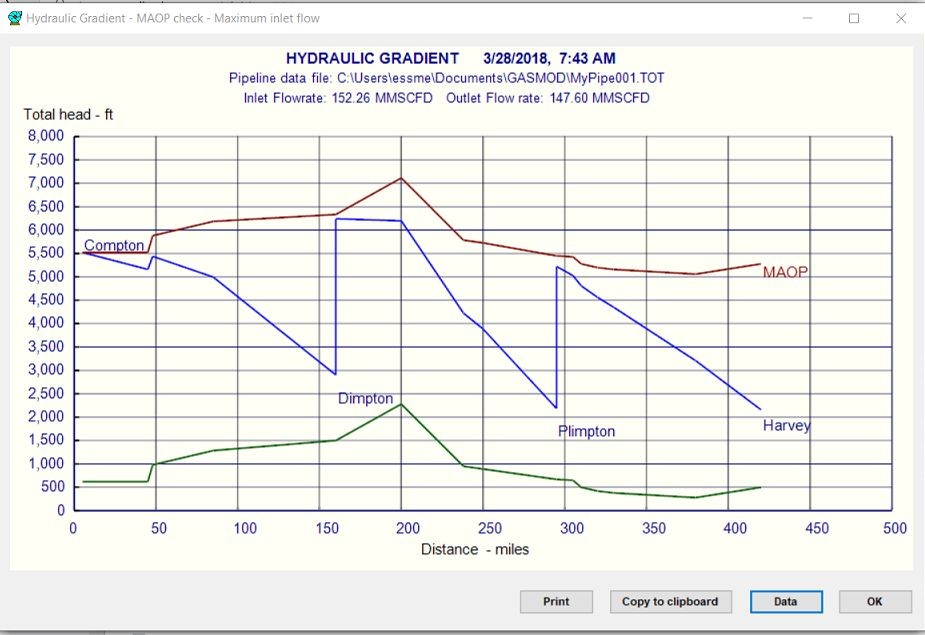
The hydraulic gradient showing the pipeline pressures superimposed on the pipeline elevation profile along the pipeline can be plotted as shown below:
Pipe Branches and Loops off the main pipeline may be modeled. Clicking the Branch menu displays the following screen. On the Branches tab, the location of the branch (main pipeline milepost), the type (IN for incoming and OUT for outgoing) of branch and the branch file name are entered in the first three columns, followed by the delivery pressure for an outgoing branch and the origin gas temperature for an incoming branch in the next two columns as shown in screen below.
To specify pipe loops, on the Loops tab, the start and end locations of the loop (main pipeline mileposts), and the loop file name are entered in the three columns.
For quick economic analyses, the capital cost and operating cost for a pipeline system can be calculated. The annual cost of service and transportation tariff can also be determined for various project financing scenarios.
Features
Use GASMOD to calculate the pipeline hydraulics, temperature and pressure profile. Despite the complexity of the program it is very user friendly. Online HELP is available for all data entry screens and the program has extensive error checking features.
Simulates steady state hydraulics of a pipeline transporting gas, considering heat transfer between the gas and the surrounding medium. Gas may be injected or delivered at various points along the pipeline.
The pipe diameter, wall thickness, absolute roughness, thermal conductivity, insulation thickness and the surrounding soil temperatures and soil thermal conductivity can all be varied throughout the length of the pipeline.
Gas may be injected or delivered at various points along the pipeline.
The gas properties, such as gravity and viscosity may be specified for each incoming gas stream. Alternatively, the gas composition (methane, ethane, etc by percent volume) may be input for each gas stream.
A database of different gas compositions may be created and saved.
The available pressure drop formulas include AGA Turbulent, Colebrook-White, Darcy-Weisbach, General Flow Equation, IGT Panhandle A & B, and Weymouth equations.
Gas compressibility factor calculation options include Standing-Katz, AGA and CNGA methods.
Several compressor stations may be located along the pipeline. The maximum discharge pressure, required minimum suction pressure and the overall compressor efficiency at each station may be specified. The final delivery pressure at the end of the pipeline may be fixed and the corresponding discharge pressure at the last compressor station computed. Alternatively, the discharge pressure at the last compressor station may be fixed and the resulting pipeline delivery pressure calculated.
Instead of a head compressor station, a pressure may be specified at the first pipe node, for a connection to another pipeline.
Compressor station fuel consumption may be calculated.
For preliminary feasibility studies, the optimum locations of compressor stations may be determined for specified Maximum Allowable Operating Pressure (MAOP) and a fixed compression ratio.
The pipeline may have branches or delivery segments of pipe. Maximum number of pipe branches is limited to 50. Each branch pipe may have up to 500 nodes compared to a maximum of 1000 nodes for the main pipeline. Currently the branch piping may not have any compressor stations.
The main pipeline may be looped. Maximum number of loops is limited to 50.
The hydraulic pressure gradient can be plotted superimposed on the pipeline elevation profile.
The capital cost of the pipeline and compressor stations and the annual operating cost for the pipeline may be calculated. This is based on specified material and labor costs and fuel gas cost for the turbine driven compressor stations. Annual cost of service and the transportation tariff for the pipeline can also be quickly calculated for economic analyses and feasibility studies.
Running the Program
A toolbar consisting of icons for commonly used menu items is available below the menu bar. These menu items or commands can be accessed by clicking on the icons. As the mouse is moved over an icon, a tool tip help appears explaining the function of each icon.
The pull down menu under File, lets you create, open, close, save or print data files. The pull down menu under Edit lets you Cut, Copy or Paste selected (highlighted) data from the spreadsheet to the Windows clipboard or from clipboard to the current cursor location in the spreadsheet. Accelerator keys, such as Ctrl-X for Cut and Ctrl-I for Insert row are available for several menu items.
The pull down menu under Options has the following :
Units - For selecting English or Metric units of calculation. Also to specify the unit of measurement for the distance along the pipeline, the pipeline flow rate and units for temperature and pressure.
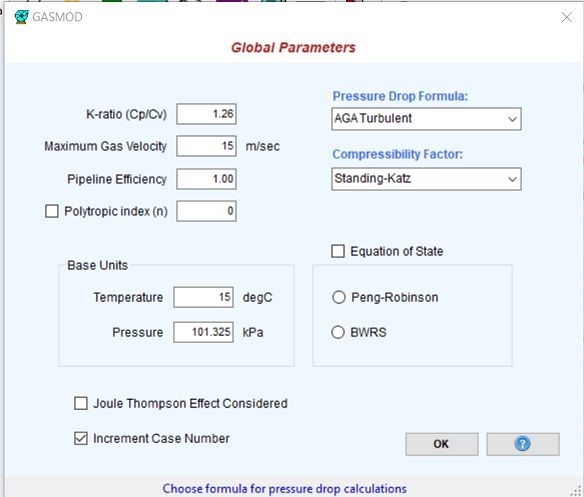
Global Parameters - This screen is used for specifying the ratio of specific heats of gas (Cp/Cv), the maximum gas velocity in the pipeline, the pipeline efficiency, the base temperature and base pressure. Also you can choose the desired pressure drop formula such as AGA, Colebrook-White, etc. and Compressibility factor method. Available options for the compressibility factor are: CNGA, Standing-Katz or AGA NX19 method. In addition, you select Joule-Thompson cooling effect in the calculations, if desired. If Joule-Thompson cooling effect is considered, less conservative results (lower pressure drop for given flow rate due to cooler gas temperatures) will be obtained. Neglecting this cooling effect will cause higher pressure drops for a given flow rate.
Interpolate Elevation - To interpolate the elevation of pipeline at an intermediate mile post.
The pull down menu under Stations has the following:
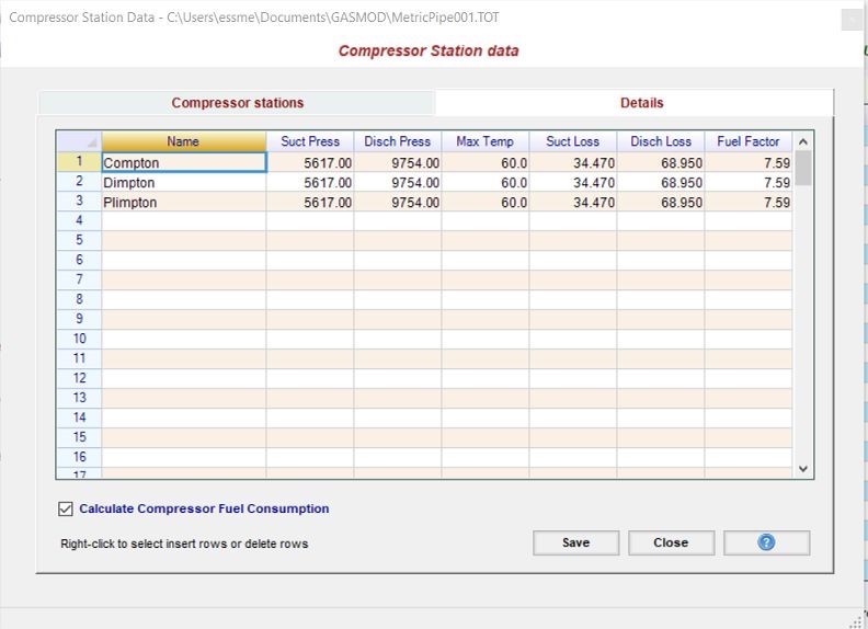
Compressor Stations - is for specifying the compressor station locations along the pipeline. The name, mile post location, status On/OFF, compressor efficiencies, mechanical efficiencies and inlet temperature are input. In addition discharge and suction pressures, maximum discharge temperature, and the suction and discharge piping losses are input in this screen. Only the suction pressure at the first compressor station is used by the program. The suction pressures at all other compressor stations are calculated for the specified discharge pressures and flow rates. At the end of the pipeline, if a particular delivery pressure is required, the discharge pressure of the last compressor station will be adjusted to provide the desired pipeline delivery pressure. To turn on this option, a check box is provided in the main pipeline spreadsheet. In addition to specifying the compressor station data, the fuel gas consumption for gas turbine driven compressors can also be calculated as an option by checking the box on the bottom left of this screen.
Locate Compressor Stations - calculates approximate locations of the compressor stations for a given MAOP and compression ratio.
Valve Stations - is for specifying Valves, and other pressure drop devices and pressure regulators. These include valves, fittings and other custom components such as meters and filters along the pipeline. The K-values needed for calculating the minor losses through valves and fittings are built into the program. You may also specify the actual pressure drop through a valve, fitting or custom device. In the latter case, the K-value is not used. To model a pressure regulator, you may indicate the downstream pressure required at a specific milepost location where the regulator will be installed.
Gas Flow - is for specifying the locations where gas enters and exits the pipeline, the gas flow rate, the inlet temperature and gas properties. The mile post location is measured from the beginning of the pipeline, the gas flow rate is positive for incoming flow and negative for a delivery out of the pipeline. The flow rate at the first mile post must always be positive, indicating inflow. The gas specific gravity (Air = 1.0) and viscosity are also input here. Alternatively, instead of the gravity and viscosity, the gas composition may be specified. Pressing the F3 key will display the available product names and gas compositions. New products can also be created and saved in the database.
The pull down menu under Branches/Loops has the following:
Branches - for entering the branch piping data. Loops - for entering the information on pipe loops.
The Graph icon is used for plotting the hydraulic pressure gradient and the gas temperature profile along the pipeline.
You can use the e-mail icon on the toolbar to send the results of calculations to a colleague or contact SYSTEK in the event of a problem with the software. The Notepad icon is to launch Windows Notepad, if you want to do some quick text editing or cut and paste results
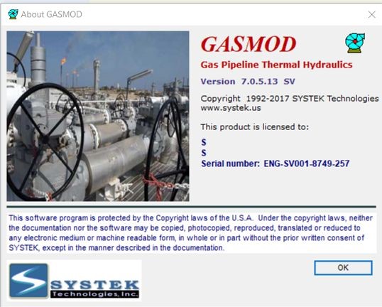
Help - provides information about the program, such as version number, user registration and general help on the program.
Sample problem:
To get a quick feel for GASMOD, run the sample problem, included with the program. Choose File/Open from the main program window. In the resulting dialog box, choose the data fileMyPipe001 The sample pipeline data file opens up. This data file contains the pipeline information for the sample problem. The calculated results are saved on disk with the default file name of MyPipe001.OUT. After viewing the results of the calculations on the screen, click OK. Click on the Print button to print the results.
Quick Pressure Drop
Upon clicking the icon with the letter "Q", the "Quick Pressure Drop: option screen opens up.
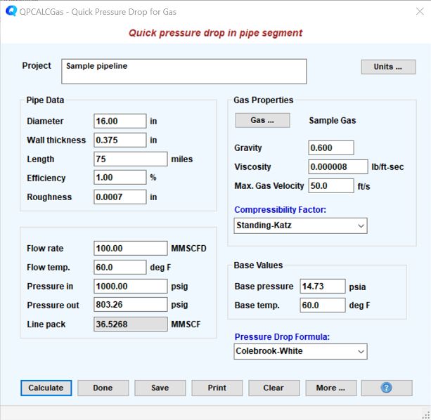
This is for quick calculation of isothermal pressure drop in a pipe segment. For a given flow rate, pipe diameter, pipe length, elevations, specific gravity and viscosity, the Quick Calc Option calculates the inlet or outlet pressure, given one of the two pressures. If the outlet pressure is specified, the inlet pressure is calculated and vice versa. You may also choose the pressure drop formula (such as Colebrook-White, General Flow Equation, Panhandle A or B etc.) to be used. By clicking the Gas button a gas composition maybe specified.
Technical Support
If you have a question about GASMOD, first refer to the Tutorial section in the User Manual, or the FAQ page at our web site (http://www.systek.us/faq.aspx). If you cannot find the answers in these places, contact SYSTEK via email or phone as described here. You must provide your program disk serial number for support. Free Technical Support is provided only during the first twelve months of the date of software purchase, to the licensed user only. After the initial free technical support period, you may elect to purchase an Annual Software Maintenance and Technical Support (SMTS) Plan. Please call SYSTEK for pricing options.
We welcome comments and suggestions from users. Please give us your thoughts on how GASMOD can be improved further. Our goal is to make this software the most user-friendly program available for engineers.
Contact SYSTEK as follows:
SYSTEK/Menon Associates, LLC.
Phone: +1(928) 733-2150
Email: support@systekus.com
Web site: www.systekus.com